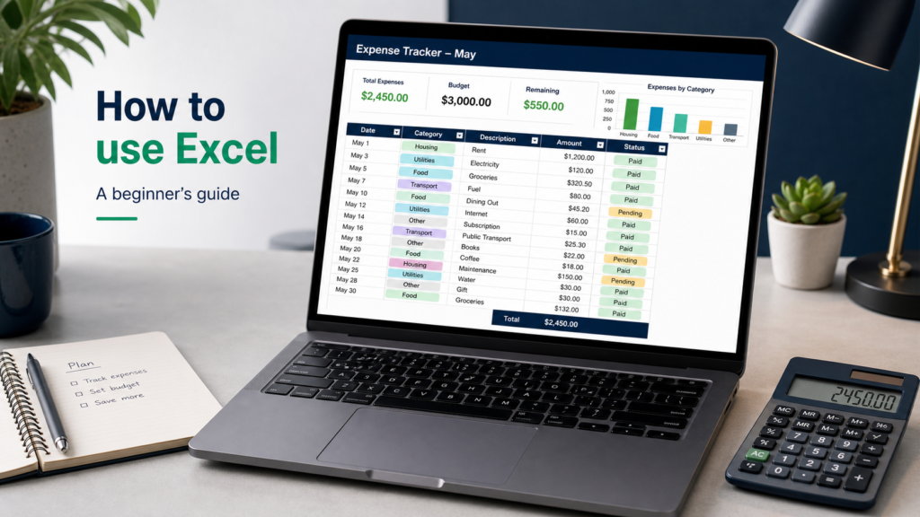
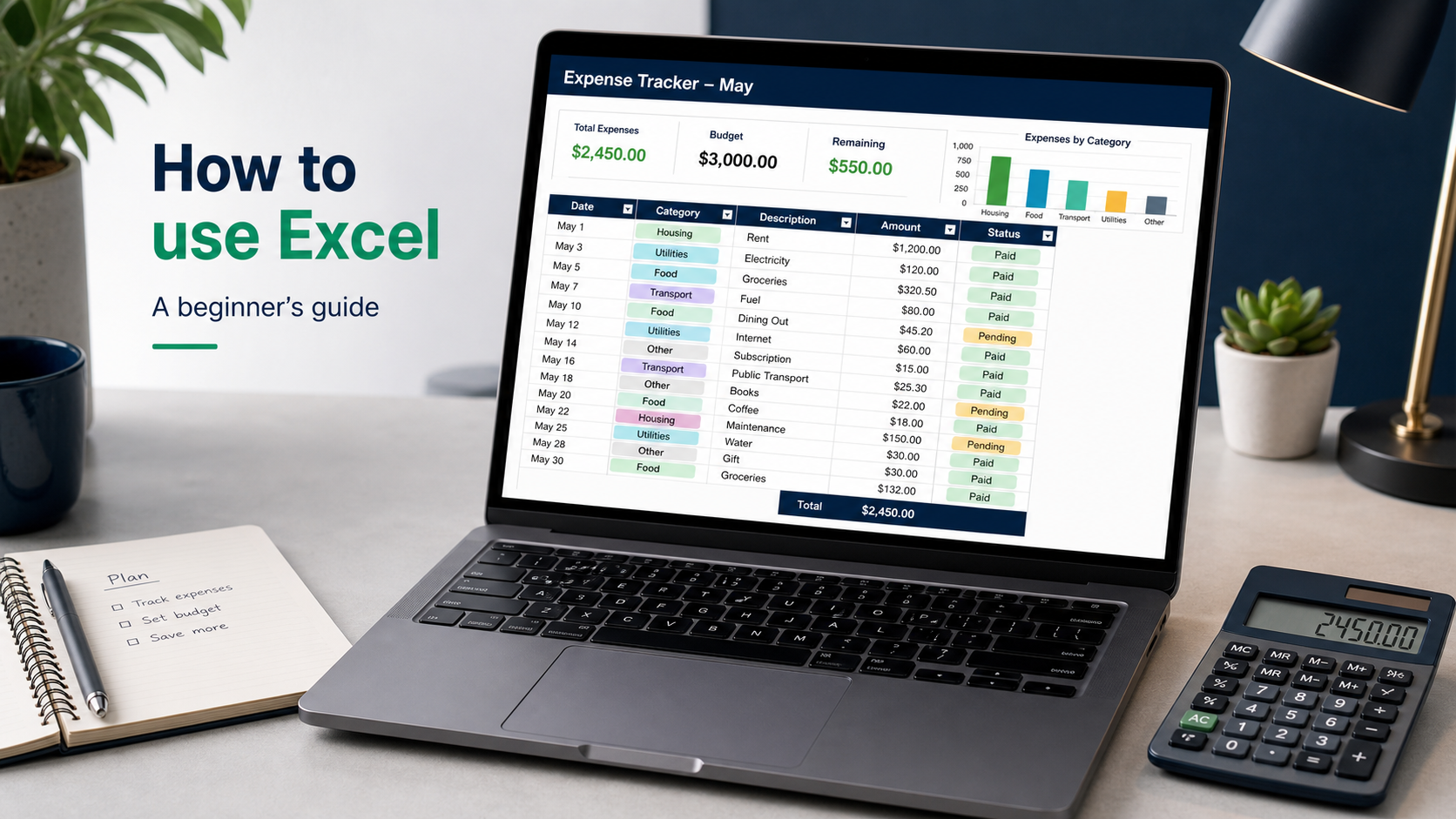
Learn Excel through one complete beginner project: turn a small expense list into a formatted table with a working total, filters, and a chart.
To use Excel, create a workbook, give each column one clear purpose, enter one record per row, format each column by data type, and start formulas with an equals sign. Convert the range to an Excel table before sorting, filtering, or charting so new rows remain part of the data.
You do not need to learn every ribbon tab first. The fastest useful lesson is to complete one small project. This guide builds a monthly expense tracker with five columns—Date, Category, Description, Amount, and Status—and turns it into a total and a category view.
Know what you are looking at
An Excel file is a workbook. Inside it are one or more worksheets, shown as tabs. A worksheet is a grid of columns labeled A, B, C and rows numbered 1, 2, 3. Their intersection is a cell, identified by an address such as D5.
The box above the grid called the formula bar shows or edits the active cell’s content. The ribbon groups commands under tabs such as Home, Insert, Formulas, Data, Review, and View. Excel for Windows, Mac, and the web may place or label a few controls differently, so use the command names in this guide rather than relying only on a keyboard shortcut.
Start with File > New > Blank workbook. Rename the first sheet Expenses so its purpose remains clear when the workbook grows.
Build one small workbook from start to finish
In row 1, type these headers:
| Cell | Header | What belongs below it |
|---|---|---|
| A1 | Date | A real calendar date |
| B1 | Category | One consistent label such as Food or Housing |
| C1 | Description | A short explanation of the expense |
| D1 | Amount | A numeric value, without words such as “dollars” |
| E1 | Status | A consistent state such as Paid or Pending |
Each later row represents one transaction. Do not create separate mini-tables for each week, place totals between records, or merge cells inside the source data. Those layouts may look organized to a person, but they make formulas, sorting, filters, and charts harder to maintain.
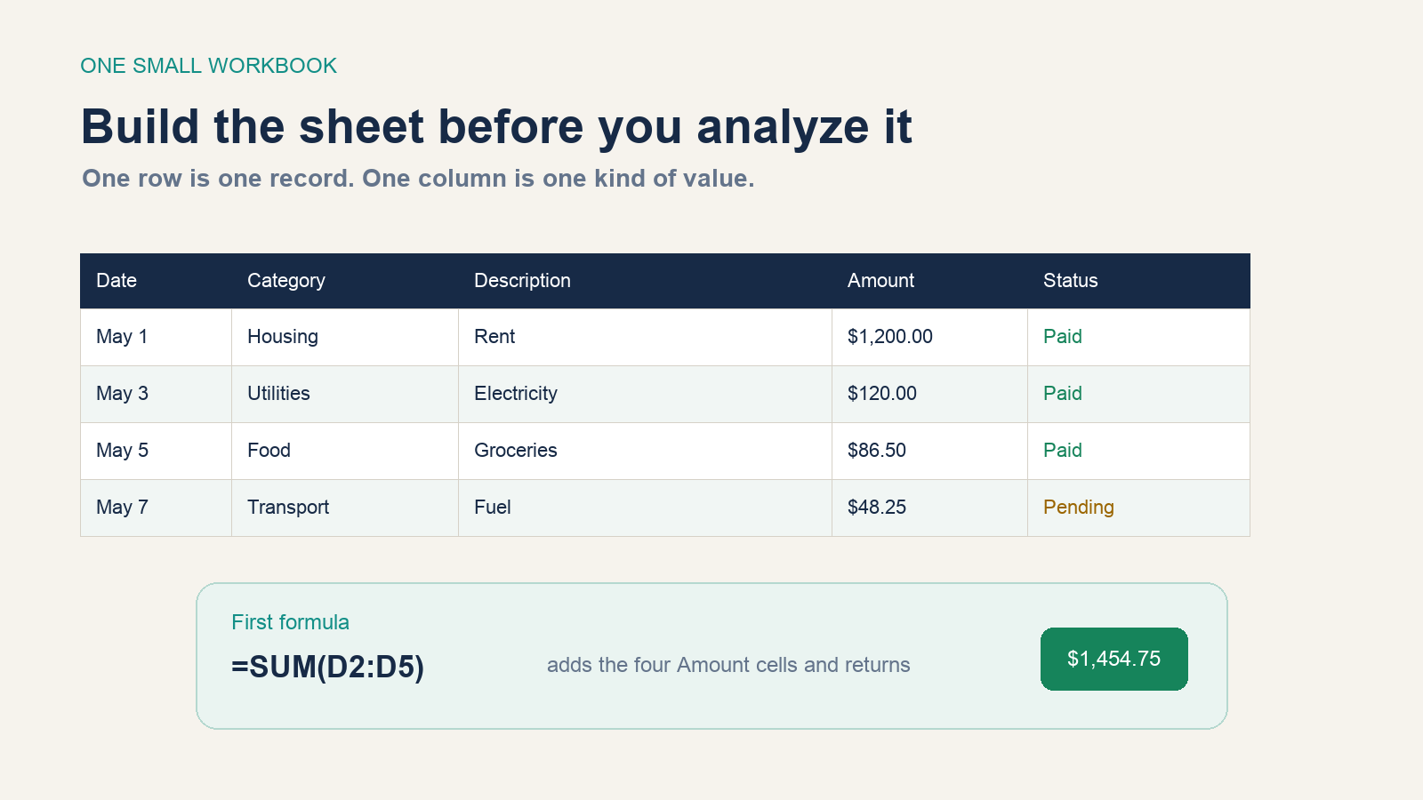
Click a cell, type a value, and press Enter to move down or Tab to move right. Microsoft’s current data-entry documentation confirms that cells can store text, numbers, dates, or times. Paste several rows when the source is trustworthy, but inspect the result rather than assuming every imported value has the right type.
Separate values, formulas, and formats
A cell has content and a display format. The number 1200 can display as $1,200.00 without storing a dollar sign as text. A date is stored as a value and can display in different date formats. This separation lets Excel calculate and sort correctly.
| Layer | Expense example | What to do |
|---|---|---|
| Value | 1200 |
Enter the amount as a number |
| Formula | =SUM(D2:D5) |
Calculate from cell values |
| Format | $1,200.00 |
Apply Currency from the Home tab |
Select column A and apply a date format. Select column D and apply Currency or Accounting. Use percentage formatting only when the stored value represents a proportion: entering 0.15 and applying Percentage displays 15%. Do not type headings such as “$ Amount” into every numeric cell.
Widen a column by dragging its header boundary or using AutoFit. Use Wrap Text for a long description. Avoid merged cells in data ranges; reserve them, if at all, for a title area outside the table.
Write your first formulas
Every Excel formula begins with =. To total the four example expenses in cells D2 through D5, select an empty cell and enter:
=SUM(D2:D5)The colon means “from D2 through D5.” Press Enter and Excel displays the result. Select that result later to see the formula in the formula bar. Microsoft’s formula overview documents the same pattern: equal sign, function, opening parenthesis, referenced range, and closing parenthesis.
You can also calculate within a row. If F1 is Budget and G1 is Difference, a formula such as =F2-D2 subtracts the expense from the budget on row 2. Drag the small fill handle at the selected cell’s lower-right corner to copy the formula down. Excel changes relative row references as it fills.
Three functions cover many first workbooks:
SUMadds values.AVERAGEreturns the arithmetic mean.COUNTcounts cells containing numbers;COUNTAcounts non-empty cells.
When a result looks wrong, inspect the referenced cells before changing the formula. A number stored as text, a blank cell, or a range that stops one row too early is often the real cause.
Convert the range to an Excel table
Click any cell in the expense range, choose Insert > Table, confirm the boundary, and keep My table has headers selected. This is not merely visual styling. According to Microsoft’s Excel table overview, a table adds header filters, expands with related new rows, can create calculated columns, and can display a totals row.
Give the table a meaningful name such as Expenses from Table Design. Table formulas can then use readable structured references. For example:
=SUM(Expenses[Amount])The range grows with the table, so the total can include new transactions without manually changing D2:D5. Microsoft’s structured-reference guidance explains how table and column names adjust as rows or columns change.
Sort and filter without breaking rows
Use the dropdown in a table header. Sort Amount largest to smallest to find the biggest transactions, or filter Status to show only Pending. A filter hides rows that do not match; it does not delete them. Clear the filter to restore the full view.
Never select one loose column and rearrange it independently from related data. Sort from inside the complete table so the date, category, description, amount, and status travel together. If numbers sort strangely, inspect whether some values were stored as text. Microsoft lists mixed types and leading spaces among common sorting problems.
Freeze the header when the list gets long: select the row below it, then use View > Freeze Panes. This affects only the view; it does not change the data.
Use the spreadsheet to answer one question
Do not insert a chart just because the button is available. Ask a question first: “Which expense categories account for the most spending?” To answer it, summarize the Amount by Category—manually for a tiny practice sheet, or later with a PivotTable—then select that compact summary.
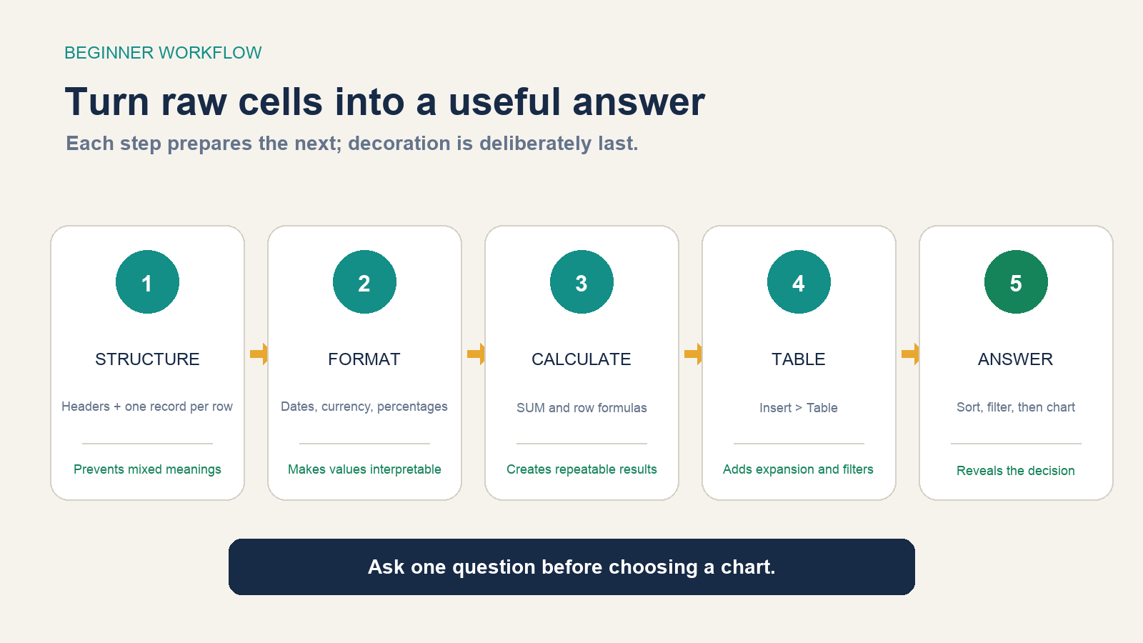
Choose Insert > Recommended Charts and preview the options. A column or bar chart is usually clear for comparing categories. Add a descriptive title such as May Expenses by Category; include data labels only when they help the reader. Microsoft’s current chart instructions likewise begin with selecting the source data, then using Insert and Recommended Charts.
If the chart looks nonsensical, repair the summary or selection instead of decorating the chart. A chart cannot correct mixed units, missing categories, duplicate totals, or dates stored as text.
Save, share, and protect the original
Press Ctrl+S on Windows or Command+S on Mac and choose a descriptive filename such as 2026-05-expenses.xlsx. Saving to OneDrive or SharePoint enables cloud access and, where supported and signed in, features such as AutoSave, Version History, and real-time collaboration. Microsoft’s save and recovery guidance explains those dependencies.
AutoSave is not a substitute for judgment. Before testing a large cleanup, unfamiliar formula, macro, or bulk paste, preserve the original or work in a copy. When sharing, remove sensitive personal data, verify permissions, and inspect hidden sheets and columns.
Your finished first workbook
You now have more than a decorated grid: a named sheet, one transaction per row, consistent columns, real numeric and date values, a working total, an expanding Excel table, safe sort and filter controls, and a chart tied to a question.
Add five of your own rows next. Confirm that the table expands, the total updates, the Pending filter still works, and the chart reflects the revised summary. If all four checks pass, you have learned the core Excel workflow and can add new functions only when a real task requires them.