

Build a six-column kg-to-lb worksheet with visible input errors, separate raw and reported values, and checked totals.
To convert a list of kilograms to pounds, divide each valid kilogram value by 0.45359237, keep that raw result, and round a separate display column. Preserve the original measurements and visibly reject invalid rows before calculating a total. The formulas below provide a repeatable worksheet method; this page is a tutorial, not an embedded converter.
For the input list 7.4, 12.8, and 23.1 kg, the results are approximately 16.3142, 28.2192, and 50.9268 lb. Together, 43.3 kg converts to approximately 95.4602 lb. If you only need one conversion, mixed pound–ounce notation, or a range, use the kilogram–pound conversion reference.
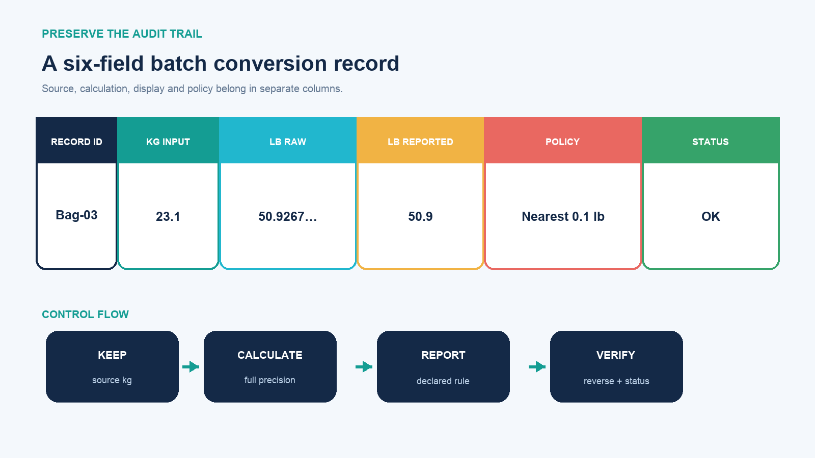
Preserve six fields for each record
Use the following column layout. Enter the numeric measurement without a suffix such as “kg”; keep the unit in the heading. The policy in this example is nearest 0.1 lb, not a carrier’s billing rule.
| Column | Heading | Purpose |
|---|---|---|
| A | Record ID | Keep the measurement attached to the correct item. |
| B | kg input | Preserve the numeric source measurement. |
| C | lb raw | Calculate pounds without an explicit rounding step. |
| D | lb reported | Round the display, leaving C intact. |
| E | Policy | Record the intended display or operational rule. |
| F | Status | Expose missing, text, negative, or error inputs. |
The NIST mass tables give the exact relationship 1 lb = 0.45359237 kg. Using division retains that factor rather than shortening its reciprocal to 2.2.
Validate the input before calculating
For an ordinary cell range in Excel or Google Sheets, start with the status formula in F2:
=IFERROR(IF(B2="","MISSING",IF(NOT(ISNUMBER(B2)),"NOT NUMERIC",IF(B2<0,"NEGATIVE","OK"))),"SOURCE ERROR")Then put this raw-pound formula in C2:
=IF(F2="OK",B2/0.45359237,"CHECK INPUT")Put the reported value in D2:
=IF(F2="OK",ROUND(C2,1),"CHECK INPUT")Fill all three formulas down through the actual imported rows. Zero remains numeric and converts to zero; a blank is MISSING. The string 23 kg, or a number stored as text, is not silently converted. Google’s ISNUMBER documentation and Microsoft’s IS-function reference distinguish numeric values from numeric-looking strings.
The status formula does not prove that a number belongs to the right item or unit. A date may also be stored as a number. Check record IDs, units, formats, and the original import; keep rejected entries for correction instead of deleting them. These rules assume nonnegative physical masses, not a signed accounting-adjustment dataset.
Choose a fill-down method for your spreadsheet
Excel calculated columns
Turn the populated range into an Excel Table with headers. Use a calculated Status column first. Microsoft explains how structured references follow table rows and columns. The lb raw column can then use the following expression; select the actual columns while editing if your headings differ:
=IF([@Status]="OK",[@[kg input]]/0.45359237,"CHECK INPUT")Use =IF([@Status]="OK",ROUND([@[lb raw]],1),"CHECK INPUT") for lb reported. Inspect the formulas in the first and final rows, then append one test record to confirm the calculated columns extend. A correct first row does not prove the entire table is covered.
Google Sheets array formulas
For the three-record example in rows 2–4, these alternatives fill each output column from one formula. Do not combine them with manually filled formulas in the same output cells. Leave the spill destinations empty.
In F2:
=ARRAYFORMULA(IFERROR(IF(B2:B4="","MISSING",IF(ISNUMBER(B2:B4),IF(B2:B4<0,"NEGATIVE","OK"),"NOT NUMERIC")),"SOURCE ERROR"))In C2:
=ARRAYFORMULA(IF(F2:F4="OK",B2:B4/0.45359237,"CHECK INPUT"))In D2:
=ARRAYFORMULA(IF(F2:F4="OK",ROUND(C2:C4,1),"CHECK INPUT"))ARRAYFORMULA expands calculations across a range. Extend every range consistently when the list grows; this example deliberately stops at row 4. It is not an automatically expanding full-column import. Formulas use English function names, decimal points, and commas as separators; adapt to your spreadsheet locale before importing real data.
Check a complete worked list
| Record | kg input | lb raw, approximately | lb reported |
|---|---|---|---|
| Bag-01 | 7.4 | 16.3142 | 16.3 |
| Bag-02 | 12.8 | 28.2192 | 28.2 |
| Bag-03 | 23.1 | 50.9268 | 50.9 |
Each row is OK. The source total is 43.3 kg and the unrounded pound total is approximately 95.46015953 lb, displayed as 95.5 lb to one decimal. Summing the separately rounded displays gives 95.4 lb. Those are different summaries and must not share an unlabeled “total.”
A larger rounding example makes the distinction clearer: ten inputs of 0.30 kg each become about 0.6613868 lb each. Round each to 0.7 lb and sum: 7.0 lb. Sum the source values first, convert 3 kg, then round once: 6.6 lb. Neither formula changes the unit factor; the order changes the report.
Block incomplete totals and reverse-check accepted rows
For the same three-row range, count accepted records with =COUNTIF(F2:F4,"OK"). Count exceptions with =ROWS(B2:B4)-COUNTIF(F2:F4,"OK"). This includes missing inputs within the expected records, rather than treating them as unused rows.
Do not publish a numeric total while any expected row is rejected. For example:
=IF(COUNTIF(F2:F4,"OK")=ROWS(B2:B4),SUM(C2:C4),"RESOLVE INPUTS")After all rows pass, compare SUM(C2:C4) with SUM(B2:B4)/0.45359237. Test individual rows with:
=IF(F2="OK",ABS(C2*0.45359237-B2)<0.000001,"CHECK INPUT")The example tolerance is 0.000001 kg for a spreadsheet round trip, not a scale-accuracy claim. Large magnitudes or a stricter application need an appropriate numerical tolerance. Protect formula columns from accidental pasting and compare first, last, and middle records, not just the grand total.
| Test input | Expected status | Expected raw result |
|---|---|---|
| 0 | OK | 0 lb |
| 0.5 | OK | About 1.10231131 lb |
| 1 | OK | About 2.20462262 lb |
| Blank | MISSING | CHECK INPUT |
| Text: 10 kg | NOT NUMERIC | CHECK INPUT |
| −1 | NEGATIVE | CHECK INPUT |
| A source-cell error | SOURCE ERROR | CHECK INPUT |
Keep calculation, operational rules, and export separate
Display formatting leaves the stored number available; ROUND creates a rounded result. NIST’s rounding guidance also distinguishes converted arithmetic from measurement precision. Keep raw results for further arithmetic, but use a governing per-item rule when the actual process requires it.
Mass conversion alone does not calculate billable shipping weight or prove a bag meets an airline limit. Do not substitute rounded pounds for the controlling unit, ignore dimensional-weight rules, or infer accuracy from extra digits. Store the applicable rule and its owner separately from the factor.
Before exporting CSV, save the formula workbook as the calculation record. A CSV handoff does not preserve this workbook’s formula logic, table behavior, validation, or formatting rules. Export clearly labeled values and units, record IDs, status, and the intended reported column; reopen the export to check row counts, decimal separators, and the total. Keep source and rejected rows recoverable.